APPLICATION OF THE OPTIMIZATION METHODS FOR THE SEARCH OF MARINE PROPULSION SHAFTING GLOBAL EQUILIBRIUM IN RUNNING CONDITION
Aleksandr Ursolov, Yuriy Batrak, Wieslaw Tarelko
Full film hydrodynamic lubrication of marine propulsion shafting journal bearings in running condition is discussed. Considerable computational difficulties in non-linear determining the quasi-static equilibrium of the shafting are highlighted. The approach using two optimization methods (the particle swarm method and the interior point method) in combination with the specially developed relaxation technique is proposed to overcome this problem. The developed algorithm allows calculating marine propulsion shafting bending taking into account lubrication in all journal bearings and exact form of journal inside bearings, compared to most of the publications that consider lubrication only in the aftmost stern tube bearing and suppose rest of bearings as pointwise. The calculation results of typical shafting design with four bearings are provided. The significance of taking into account lubrication in all bearings is shown, specifically more exact values of bearings’ reactions, shafting deflections, minimum film thickness and maximum hydrodynamic pressure in the stern tube bearing in case of considering lubrication in all bearings.
Keywords: marine propulsion shafting, bearing lubrication, fluid-structure interaction, finite-element method, optimization
INTRODUCTION
FORMULATION OF THE PROBLEM
Bearings are one of the most important parts of a ship’s propulsion system. Therefore, at the design stage, it is crucial to ensure whether bearings and especially an aft stern tube bearing operate properly under the specified operational conditions (propeller loads, ship motions at the rough sea, hull deflections etc.). For this, it is necessary to have reliable information about the interaction between the shafting and bearings, which are spatially positioned in a certain way. The spatial location of the bearings is achieved through the shaft alignment procedure, which is vital for the shaft line safe operation. Improper shafting alignment could lead to the lack of hydrodynamic lubrication and cause the rapid temperature rise, whipping, melting or burning of non-metallic bearing bushes during manoeuvring or even normal operation. To determine the optimal bearing positions, it is necessary to be able to reliably and effectively calculate the static equilibrium of the shaft line with regard to lubrication. More precisely, it is a quasi-static equilibrium because it comes about the running shafting. The external loads applied to the operating shafting are averaged and considered as constant, shafting vibration being neglected.
The determination of the interaction between the shafting and bearings in operation belongs to the non-linear fluid-structure interactions class of problems (FSI). To solve it, a number of solutions are to be found: shafting elastic bending, lubrication for each of the shafting’s bearings and elastic deflections of bearing bushes, which is essential for water lubricated bearings with non-metallic bushes [10, 11] (the latter is beyond the scope of the present paper).
The complexity of the concerting the listed tasks solutions is caused by the fact that in properly lubricated bearings, the shaft is lifted by the developed hydrodynamic pressure which depends on the lubrication film thickness. In turn, the lubrication film thickness is determined by the journal position and curvature (the aft stern tube bearing has a high \(\displaystyle {L/D}\) ratio,
therefore, the journal curvature should not be ignored since it affects hydrodynamic pressure considerably). Furthermore, the position of the journal is unknown before calculation as well as hydrodynamic pressure distribution. Therefore, shafting deflections and hydrodynamic pressure depend on each other and iterative techniques should be applied to this FSI problem in order to find the static equilibrium position of the system.
LITERATURE REVIEW
The paper subject is not new and has been presented by the other authors in similar formulations. However, some of them consider lubrication of the stern tube bearing only, some use simplified lubrication models and some do not clarify the method of the global equilibrium search.
Mourelatos and Parsons [12] presented the method for determining equilibrium position of the shafting with the water lubricated aft stern tube bearing but the rest of the bearings are considered as non-lubricated pointwise supports. The divergence nature of the shafting-bearings system which fails successive numerical simulation is illustrated and the optimization based approach for the equilibrium search is introduced. The deformation of bearings’ bushes is taken into account.
Vulic [20] highlighted the importance of considering lubrication fluid film in shaft alignment design in contrast to the commonly used approach to neglect it. He presented the method to find equilibrium position of shafting taking lubrication into account, however bearing model is represented by approximation of Reynolds equation solution for bearing with relative length of \(\displaystyle {0 < L/D \leq 2}\) so any modifications of bearing surface (wear, double sloping etc.), elastic deflection of polymer or rubber bush and journal bending inside bearing cannot be taken into account. The difficulties in the convergence of successive iteration approach are also mentioned.
Xing and et al. [25] consider the behaviour of the marine propulsion shafting using Multi-Body Dynamics approach that implemented in ANSYS software. Lubrication of the bearings and bearing bush elastic deflections have been considered and it has been shown that investigation of the marine stern tube bearings lubrication should be performed taking journal curvature into account. Unfortunately, no method’s or its convergence details has been presented in the paper.
Similarly, Andreau et al. [1] stated that they solved the global equilibrium problem taking bush elastic deflections into account by means of the iterative procedure, but no clarification of an equilibrium search method and its convergence have not been done.
Gurr and Ruifs [6] consider lubrication based on the Reynolds equation solving only for the aft stern tube bearing, the other bearings were being represented by the simplified lubrication model neglecting misalignment. The used iterative scheme also is not discussed.
There are also papers, e.g. [7, 5 , 24, 25] that only consider isolated perfectly aligned isolated bearings and provide calculation methods for journal eccentricity and attitude angle without global shafting equilibrium.
Hirani et al. [7] provide a rapid method determining design parameters of the bearing taking into account oil flow and temperature effects. The heuristic closed form solution of the Reynolds equation is used for determining pressure distribution.
Kraker et al. [5] presented the computational method of solving the mixed elastohydrodynamic problem. The iterative secant method is used to find the eccentricity of the journal and the pseudo-dynamic stepping is used to prevent numerical instability of the staggered scheme between Reynolds equation and bearing bush deformation through introducing artificial damping in the structure.
Xie et al. [24, 25] provide a Stribeck curve calculation method and investigate the influence of the main bearing design parameters on it. Three models of bearing performance for boundary lubrication, mixed lubrication and hydrodynamic lubrication regimes are considered.
From the above, it follows that, despite the fact that many researchers dealt with the described problem, there are no generally accepted reliable method which fully would meet the authors’ requirements.
METHOD
In the proposed method, the journals’ and bushes’ local deflections under the hydrodynamic pressure are not considered. While ignoring the journal local deflection is a commonly used hypothesis, ignoring bush deflections is valid only for metal bearings bushes. The algorithms for polymer and rubber bearings elastohydrodynamic modelling that take local elastic bush deflections are under development now.
The method also restricted by only pure hydrodynamic lubrication and do not consider any solid contact between the journal and bearing bush.
SHAFT BENDING
The shafting elastic deflections are determined by solving the system of linear algebraic equations of the finite element method (FEM) for the beam theory
where \(\displaystyle {[K]}\) is a stiffness matrix of the shafting; \(\displaystyle {\{ u \}}\) is a nodal displacement vector; \(\displaystyle {\{ q_{w} \}}\) is a vector of the weight loads; \(\displaystyle {\{ q_{p} \}}\) vector of the propeller hydrodynamic loads; \(\displaystyle {\{ q_{l} \}}\) is a vector of loads from the hydrodynamic pressure that is unknown initially and to be found iteratively. The coordinate system accepted in the present paper is the follows: the initial point at the aft end of a shafting; \(\displaystyle {x}\)-axis is directed forward along shafting; \(\displaystyle {y}\)-axis is directed to the port side; \(\displaystyle {z}\)-axis is directed upward.
The Timoshenko beam element stiffness matrix [14] is used. It was reduced to take into account only lateral liner and angular displacements in the vertical and horizontal planes. Shear area coefficient for the beam element with the circular transverse section is calculated according to the recommendations [8].
LUBRICATION
The Reynolds equation [19] for lubrication under full hydrodynamic regime is solved numerically
where \(\displaystyle {h(x, y)}\) is lubrication film thickness, m; \(\displaystyle {p(x, y)}\) is hydrodynamic pressure, Pa; \(\displaystyle {U=0.5 d \omega}\) is linear velocity of the journal surface, m/s; \(\displaystyle {d}\) is journal diameter, m; \(\displaystyle {\omega}\) is journal spin speed, rad/s. In Eq. (2), the \(\displaystyle {x}\)-axis is directed along bearing and the \(\displaystyle {y}\)- axis is directed around the bearing bush circumference. The procedure presented in book [15] was applied to Eq. (2) in order to derive the stiffness matrix of the lubrication film finite element. The temperature and viscosity of the lubricant are supposed to be defined and constant throughout the lubrication film. Despite the fact that viscosity and temperature variations of the lubricant are important for journal bearing load caring capacity, they are assumed to be defined and constant throughout the lubrication film for simplicity. The viscosity variation effect will be considered in further researches.
Although FEM allows setting arbitrary bush shape, for simplicity, the only grooveless cylindrical bush surface was considered. Lubrication film thickness is defined as follows:
where \(\displaystyle {\Delta}\) is bearing diametrical clearance, m; \(\displaystyle {e(x)}\) and \(\displaystyle {\varphi_e(x)}\) eccentricity and attitude angle of journal, respectively. Position of the journal depends on the spatial position of the shafting and bearing
where \(W_y(x)\) and \(W_z(x)\) are shafting deflections, \(w_y\) and \(w_z\) are lateral bearing axis offsets, \(\alpha_z\) and \(\alpha_z\) are angular bearing axis slope, \(x_c\) is the longitudinal position of the bearing length’s middle.
After solving Eq. (2), the pressure is integrated at the circular direction and then transformed to nodal loads in the vertical and horizontal planes to be applied to the journal.
OPTIMIZATION
The static equilibrium of the shafting is reached when sums of all forces and moments acting on the shafting are equal to zero:
The possible way to fulfil these conditions is described below. Following the method [12], the auxiliary pointwise support is introduced in the middle of each bearing that allows solving the shafting bending equations. The support position in the transverse section can be specified by non-dimensional cylindrical coordinates
where \(\displaystyle {\overline e}\) is non-dimensional eccentricity, \(\displaystyle {\overline {{{\rm{\varphi }}_e}}}\) is non-dimensional attitude angle. When the pressure distribution in the bearings corresponds to the shafting equilibrium position, reactions of all auxiliary supports in the vertical and horizontal planes are to be equal to zero as if the auxiliary supports have disappeared. Therefore, fulfilment of the first condition of equilibrium Eq. (2) could be represented as the following optimization problem:
where \(\displaystyle {{\widetilde{R}_j}}\) is the reaction of the \(\displaystyle {j}\)-th auxiliary support, \(\displaystyle {\widetilde{R}_{z{\rm{ }}j}}\) and \(\displaystyle {\widetilde{R}_{y{\rm{ }}j}}\) are its vertical and horizontal projections, is the number of lubricated bearings in the system. The general number of variables \(\displaystyle {X}\) is twice a number of lubricated bearings in the scheme.
It should be mentioned that in [12], the objective function is based on the minimizing difference between journal deflections in two positions: when it is fixed by the auxiliary support and when it is supported only by hydrodynamic pressure. However, this approach is unacceptable in the case of several lubricated bearings, because at least two bearings have to be considered as fixed pointwise supports without lubrication in order to provide constraints for the shafting finite element model. Moreover, the deflections in contrast to bearing reactions are not integral values so this approach cannot provide stable convergence of the iterative procedures when lubrication of several bearings is considered.
It is well known that there is no universal best optimization method but there are methods that are most applicable to the certain problem. To find an appropriate method to solve this problem, a number of optimization methods (such as interior point method, trust region method, sequential quadratic programming, active set method, Nelder-Mead simplex algorithm, Hooke-Jeeves or pattern search, genetic algorithm, simulated annealing, particle swarm method) were tested. It was found that the interior point method and the particle swarm method are the most appropriate for this problem. The particle swarm method [9, 13, 18] is effective for searching approximate global minimum, but it is too slow for searching the final result. In contrast, the interior point method [4, 21, 22] searches the minimum of the function successfully and fast, but only if the initial point of optimization is close to the solution point. Therefore, the sequential application of these two methods proved to be the most effective in this case. It is significant that advantage of the particle swarm method use at the first stage is growing with the growth of a lubricated bearings number in the calculation and there is no need to use it in the case of one lubricated bearing in the scheme, e. g. only an aft stern tube bearing. When a number of similar calculations should be done (e. g. different rotation speeds) then the auxiliary supports’ position from the previous solution could be used as an initial point for the new one without preliminary using the particle swarm method that significantly speeds up the calculation.
The solution of the optimization problem is satisfactory if the objective function \(F(x) < 0.01\) N . Otherwise, bearing auxiliary supports remain loaded and equilibrium purely due to hydrodynamic pressure is not reached. It was found during testing different cases that it is enough to use 20 particles and 20 iterations of the particle swam method in order to localize the objective function minimum.
RELAXATION TECHNIQUE
In the applied approach, auxiliary support fixes the position of journal centre point in space but the journal can freely rotate relative to this point so optimization can meet only the first condition of equilibrium Eq. (8). Applying the optimization methods to fulfil conditions Eq. (8) and Eq. (9) simultaneously leads to a significant increase in the variables number that makes such an approach not effective for practical use. The fact is that moments generated by the hydrodynamic pressure relative to auxiliary support point are very sensitive to a journal angular position and this relation is highly nonlinear, especially for bearings with high \(\displaystyle {L/D}\) ratio.
Therefore, the special relaxation approach was developed in order to reach convergence in the searching shafting equilibrium including condition Eq. (9). The proposed relaxation is in somewhat similar to the pseudo-dynamic approach in [5]. However, the present method simulates not only damping but also inertia in order to avoid looping. The procedure uses two previous pressure distributions to correct the pressure in the current iteration, that is to be applied to the journal:
where \(\displaystyle {p_i}\) is pressure that calculated at present iteration; \(\displaystyle {p_{i – 1}}\) and \(\displaystyle {p_{i – 2}}\) are two previously used corrected pressures.
The weight coefficients , \(\displaystyle {{C_1}}\), \(\displaystyle {{C_2}}\) and and \(\displaystyle {{C_3}}\) are derived from the following conditions:
– Coefficient \(\displaystyle {{C_1}}\) is the main and determines the part of the directly calculated pressure at the present iteration. For stabilization at the initial critical steps, it increases linearly up to set \(\displaystyle {{C_1}(n)}\) value and after that remains constant.
– Coefficients \(\displaystyle {{C_2}}\) and and \(\displaystyle {{C_3}}\) that correspond to the parts of the pressure at two previous iterations have a constant relative proportion.
– Coefficients \(\displaystyle {{C_1}}\), \(\displaystyle {{C_2}}\) and and \(\displaystyle {{C_3}}\) are set that the sum of them are to be equal one: \(\displaystyle {{C_1} + {C_2} + {C_3} = 1}\).
The coefficients derived from the mentioned conditions are as the following:
The dependences Eq. (16)-(18) can be fully defined by the parameters \(\displaystyle {{C_1}(2)}\), \(\displaystyle {{C_1}(n)}\), \(\displaystyle {n}\) and \(\displaystyle {{C_2}/{C_3}}\), that are constant for the algorithm and were found from the systematic calculations of different shafting models.
The cycle of equilibrium search is ended if one of the conditions is fulfilled:
– moments of corrected pressure \(\displaystyle {p_i^*}\) for each bearing relative to the corresponding auxiliary supports’ points in the vertical \(\displaystyle {M_y}\) and horizontal \(\displaystyle {M_z}\) planes differ from the values at the previous iteration and from non-corrected moments of the pressure calculated at the present iteration by the value lesser than acceptable error \(\displaystyle {\Delta M}\);
– an iteration number \(\displaystyle {i}\) is more than set maximum \(\displaystyle {i_{max}}\).
The latest condition provides end of the cycle to stop the current optimization step and start a new one.
These conditions could be written as
where \(\displaystyle {\wedge}\) and \(\displaystyle {\vee}\) are AND and OR logical operators, \(\displaystyle {M_y}\) and \(\displaystyle {M_z}\) are determined as:
Unlike the other papers, at each step of the cycle, the calculation is performed for every lubricated bearing so that equilibrium is found iteratively taking interaction between bearings into account. This interaction impacts the exact journal positions and pressure and ignoring it could lead to incorrect results.
APPLICATION OF THE METHOD
The presented method is illustrated by the calculation of a somewhat simplified typical shafting design with four lubricated bearings. The shafting scheme and dimensions are illustrated in Fig. 1, shaft diameter \(\displaystyle {d = 0.5}\) m is constant along the shafting and the four-blade propeller with diameter\(\displaystyle {D = 5.6}\) m is located at \(\displaystyle {x = 0.7}\) m. Shafts are made of steel with following properties: elastic modulus \(\displaystyle {E=2 \cdot 10^4}\) MPa, Poisson ratio \(\displaystyle {\nu=0.3}\), density \(\displaystyle {\rho = 7850}\) kg/m3. General parameters and mesh discretization of the bearings are listed in Table 1.
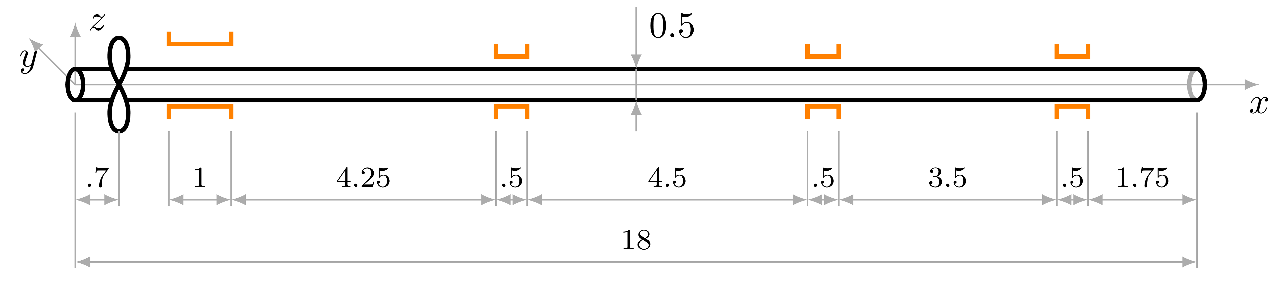
Fig. 1. Dimensions of the shafting model (in meters)
Tab. 1. General characteristics of the bearings
| Bearing | Length | Clearance | Viscosity | Long. grid step | Circ. grid step |
| number | \(\displaystyle {\Delta}\), m | \(\displaystyle {\Delta}\), mm | \(\displaystyle {\mu}\), Pa s | \(\displaystyle {dx}\), m | \(\displaystyle {d\varphi}\), deg. |
| 1 | 1 | 0.8 | 0.02 | 0.025 | 2 |
| 2, 3, 4 | 0.5 | 0.4 | 0.02 | 0.05 | 4 |
Hydrodynamic propeller loads significantly impact the shafting bending and, therefore, the bearing pressure. The propeller loads highly depend on the so the developed method should be able to find the solution (if it exists) for different s. According to the article [3], mean values of the propeller loads can be defined as:
where \(\displaystyle {P_x}\) and \(\displaystyle {M_x}\) are thrust and torque correspondingly (N and Nm), their values being depended on rotational speed. Calculations have been performed for rotational speeds range from 60 to 120 \(\displaystyle {rpm}\) with the step of 20 \(\displaystyle {rpm}\).
In order to assess the effect of bearings lubrication on the stern tube bearing performance, two types of calculation were provided:
– all bearings are considered as lubricated;
– only the aft stern tube bearing is considered as lubricated.
The shafting is loaded by:
1. the distributed shaft weight \(\displaystyle {q = -0.25 \, d^2 \, \pi \, \rho \, g = -15.1}\) kN/m, where \(\displaystyle {g=9.81}\) m/s2 is the acceleration of gravity;
2. concentrated propeller weight taking buoyancy into account \(\displaystyle {P_w = -127.5}\) kN;
3. hydrodynamic propeller loads, listed in Table 2.
Tab. 2. Hydrodynamic propeller loads
| \(\displaystyle {rpm}\) | \(\displaystyle {P_x}\), kN | \(\displaystyle {P_y}\), kN | \(\displaystyle {P_z}\), kN | \(\displaystyle {M_x}\), kNm | \(\displaystyle {M_y}\), kNm | \(\displaystyle {M_z}\), kNm |
| 60 | 210.8 | 10.5 | 10.1 | 198.9 | 69.6 | 56.5 |
| 80 | 374.7 | 18.7 | 18.0 | 353.7 | 123.8 | 100.4 |
| 100 | 585.5 | 29.3 | 28.1 | 552.6 | 193.4 | 156.9 |
| 120 | 843.1 | 42.2 | 40.5 | 795.8 | 278.5 | 226.0 |
RESULTS AND DISCUSSION
The calculation has been performed at each rotation speed using both optimization methods when lubrication of all bearings is considered and using only the interior point method when only the stern tube bearing is considered as lubricated. The number of iterations for each of the method and total objective function calls are listed in Table 3. As expected, in the case of considering all bearings as lubricated, the iteration number is greater than in the case when only the aft stern tube bearing is considered as lubricated due to the growth of variables number in optimization. It should be mentioned that when only the interior point method was applied to the case considering lubrication in all bearings, no solution has been found. This highlights the importance of using both optimization methods when several bearings are considered as lubricated.
Tab. 3. Computational effort
| All bearings | Only aft stern tube bearing | |
| Particle swam, iterations | 20 | 0 |
| Interior point, iterations | 56…70 | 24…30 |
| Objective function calls | 1147…1430 | 109…130 |
The hydrodynamic pressure moment convergence when the simple successive iterations and proposed relaxation method is shown in Fig. 2. It can be clearly seen that the simple successive approximations (see Fig. 2a) haven’t converged whereas pressure relaxation Eq. (15) accurately determines journal angular position (see Fig. 2b). It shows the efficiency of the relaxation method.
Fig. 3 shows hydrodynamic pressure in the stern tube bearing at the different speeds in the case of all lubricated bearings. There are significant pressure peaks at 60 and 120 \(\displaystyle {rpm}\) (Fig. 3d and 3a) caused by edge loading. It indicates that the method can be used in any possible hydrodynamic pressure distributions. The dependencies of maximum pressure \(\displaystyle {p_{max}}\) and minimum lubrication film thickness \(\displaystyle {h_{min}}\) in the stern tube bearing on are illustrated in Fig. 4. As can be expected, with the decreasing of minimum film thickness, the maximum pressure in the bearing becomes greater. It should be noted that ignoring lubrication of the intermediate bearings have led to the error in maximum pressure in stern tube bearing of 30% in case of the aft edge loading (60 \(\displaystyle {rpm}\)) and 22% in case of the forward edge loading (120 \(\displaystyle {rpm}\)). It illustrates the importance of considering lubrication of all bearings.
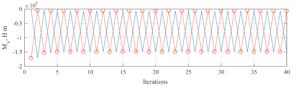
a. without relaxation
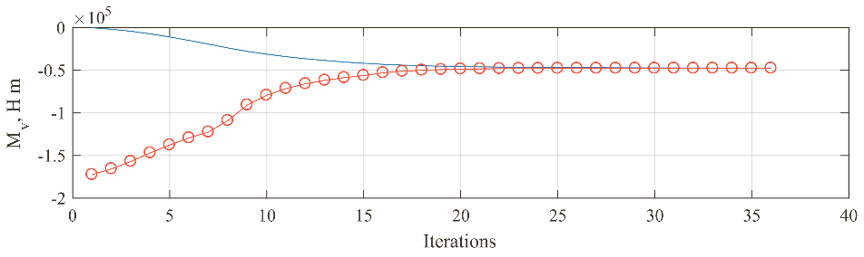
b. with relaxation according to Eq. (11)
Fig. 2. Stern tube vertical moment convergence plot: (––o––) is moment by directly calculated pressure , (–––) is moment by corrected pressure
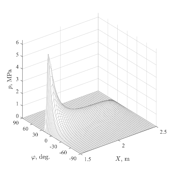
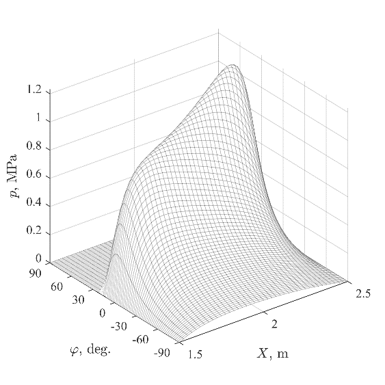
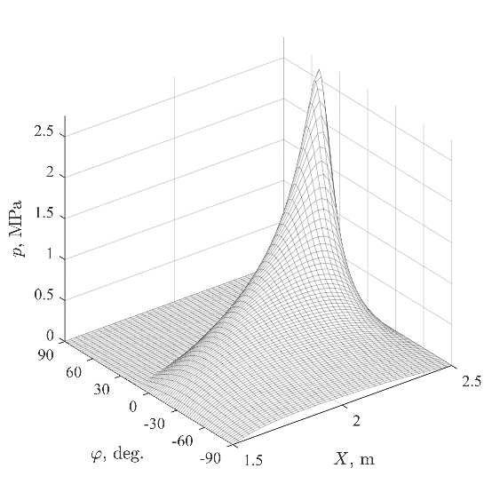
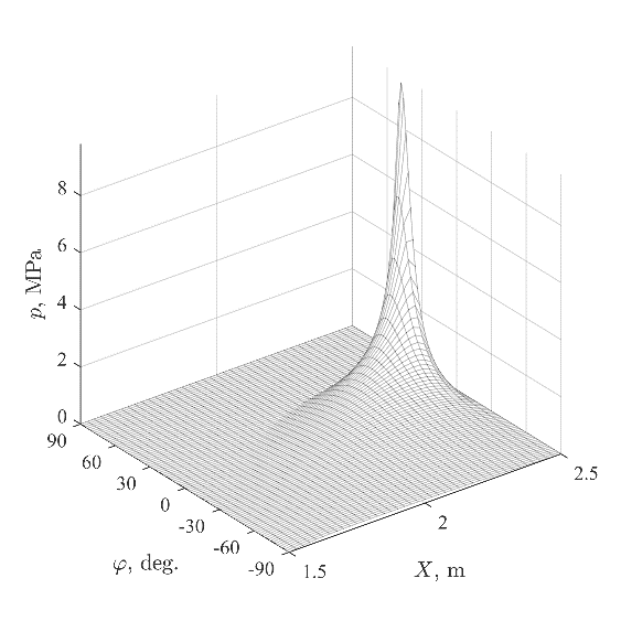
Fig. 3. Hydrodynamic pressure in the aft stern tube bearing
The eccentricity distributions of the bearings’ journals at the different speeds are illustrated in Fig. 5. The propeller loads cause a significant misalignment in the stern tube bearing, a small journal slope in the second bearing and almost no slope in other bearings. It should be noted that slope sign is changed with the growth of \(\displaystyle {rpm}\).
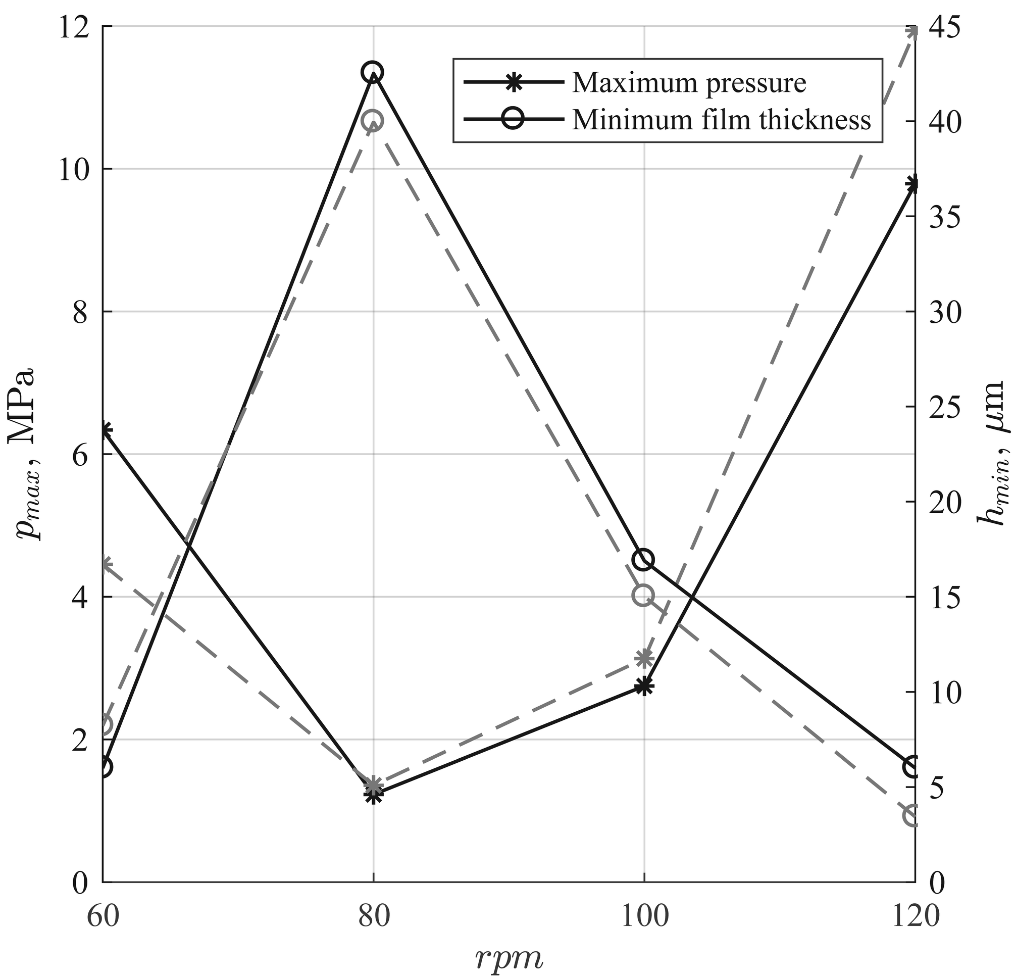
Fig. 4. Characteristics of the aft stern tube bearing: (–––) is for all lubricated bearings, (- -) is for the aft stern tube lubricated bearings only
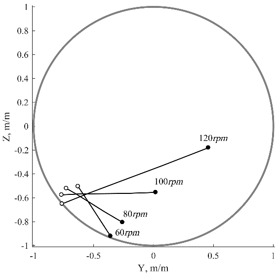
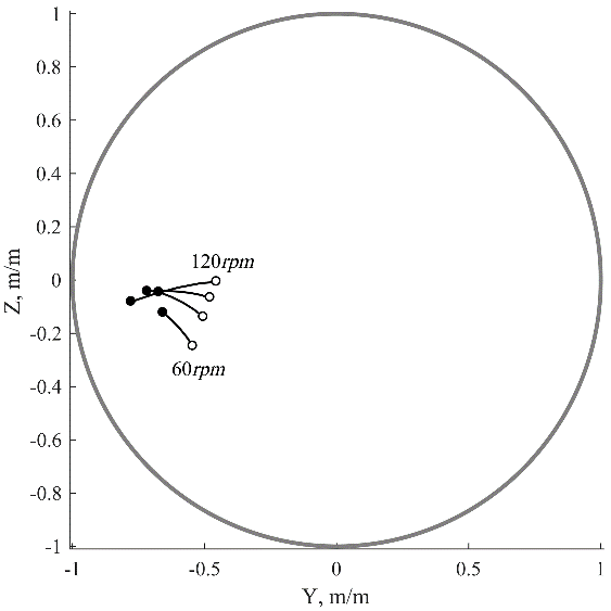
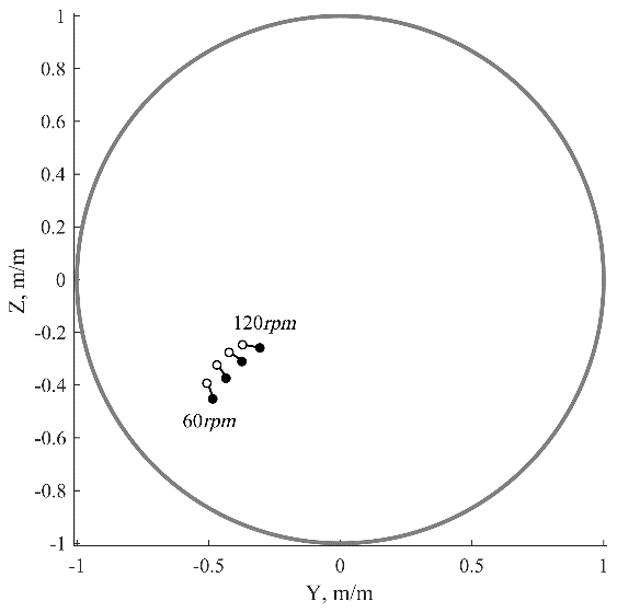
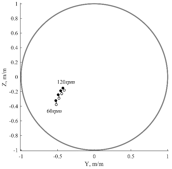
Fig. 5. Journal position inside bearings clearance circle: – at the fore bearing edge, – at the aft bearing edge
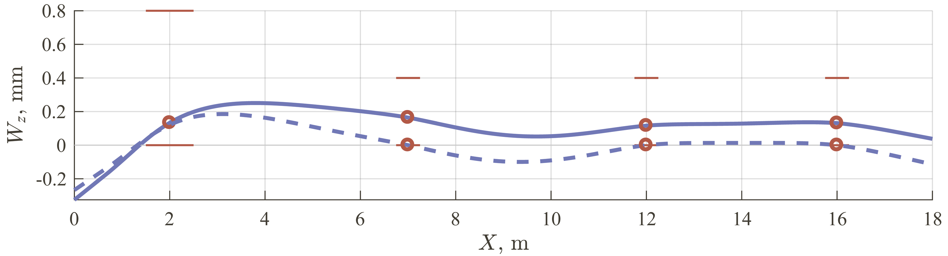
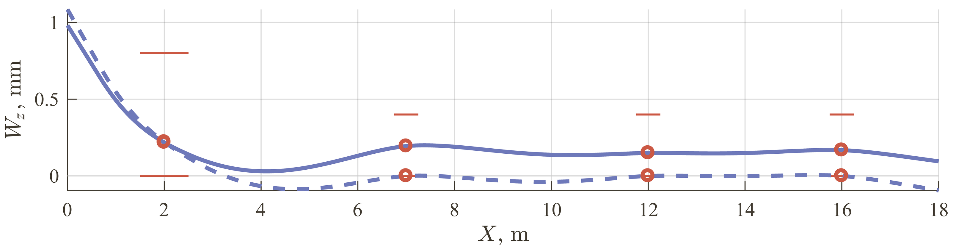
The deflections of the shafting at 60 and 120 \(\displaystyle {rpm}\) in the vertical plane and horizontal plane are shown in Fig. 6 and Fig. 7 correspondingly. The solid lines correspond to the shaft deflections in the case of all lubricated bearings and dashed lines in the case when only stern tube bearing lubrication is considered. The shaft deflection magnitudes rise in the horizontal plane and journal slope sign changes in the vertical plane because of the propeller loads increase with the rotational speed increase. It should be noted that ignoring lubrication in the intermediate bearings leads to changes in the shafting deflections and the corresponding position of the aft stern tube bearing journal up to 4% of its diametric clearance so the estimation of shafting operation could be incorrect.
The bearings reactions \(\displaystyle {R}\) are depicted in Fig. 8 and one can see that with the rise of , load redistribution occurs between 1-st and 2-nd bearings so that reaction on the 2-nd one increased two times from 60 to 120 \(\displaystyle {rpm}\). However, reactions of the third and fourth bearings changed little.
a. 60 \(\displaystyle {rpm}\)
b. 120 \(\displaystyle {rpm}\)
Fig. 6. The vertical projection of the shaft deflections: (–––) is for all lubricated bearings, (- -) is for aft stern tube lubricated bearing only
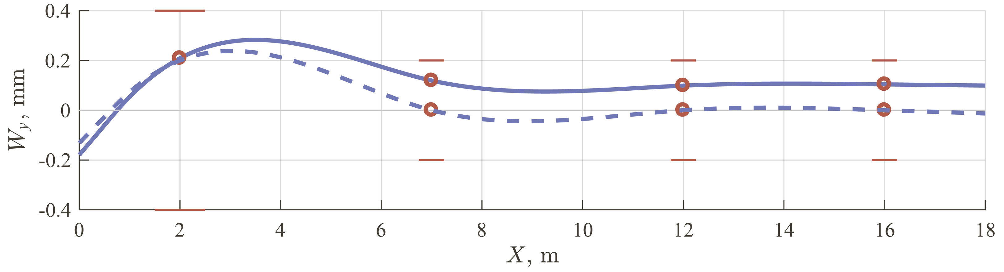
a. 60 \(\displaystyle {rpm}\)
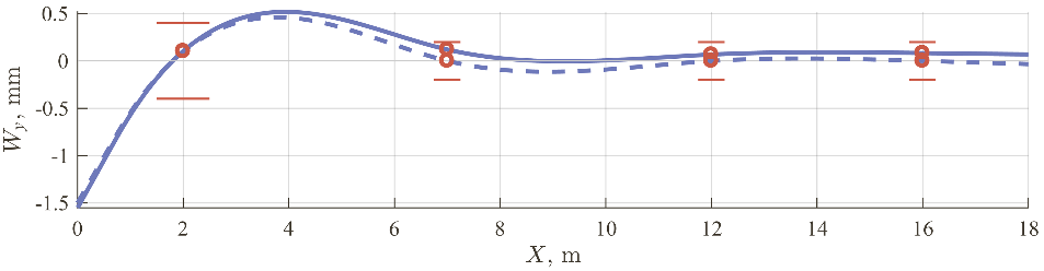
b. 120 \(\displaystyle {rpm}\)
Fig. 7. The horizontal projection of the shaft deflections: (–––) is for all lubricated bearings, (- -) is for aft stern tube lubricated bearing only
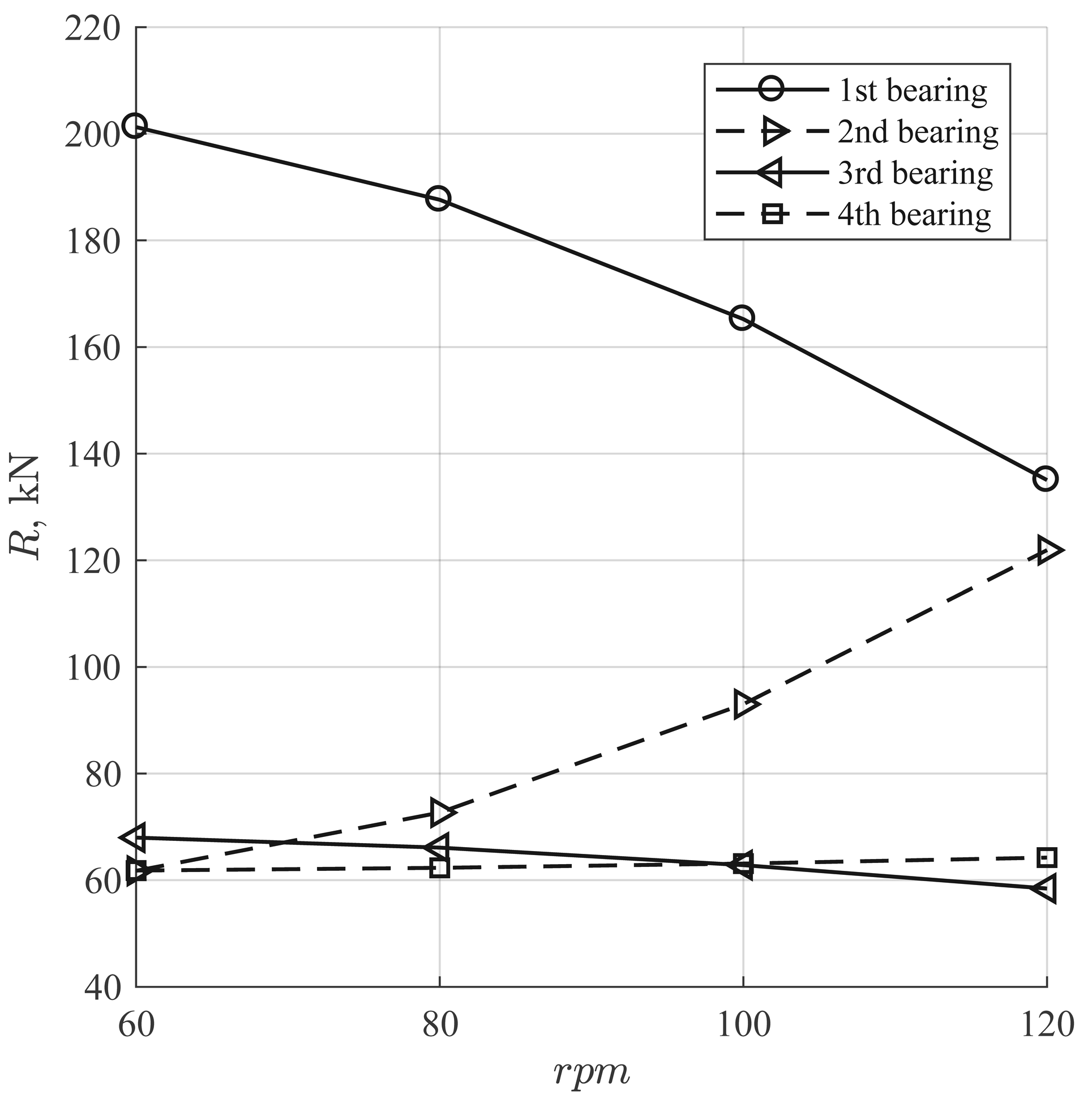
Fig. 8. Bearings reactions
CONCLUSIONS
The proposed method allows performing propulsion shafting static calculation taking into account a number of lubricated bearing in the model affecting each other even if significant journal slope and bearing edge loading takes place. The method is free of assumptions such as the constant slope of the journal, pointwise representation of the intermediate bearings, restrictions of \(\displaystyle {L/D}\) ratio and bearing surface cylindricity. Thereby, it allows a designer to perform the deep precise analysis of the system and more qualitative offset optimization at the design stage. It should be mentioned that reliable determination of the aft stern tube bearing lubrication is essential for providing its reliability and performance prediction.
In such a FSI calculation, the convergence is the most challenging issue. The method is based on the optimization approach and thus provides the stable loopless convergence of the journal linear position. However, due to the adopted approach with auxiliary artificial support, the additional cycle is required to find the angular position of the bearing journals. The developed relaxation technique provides stable convergence between angular journal positions and hydrodynamic pressure so that not only the force equilibrium condition but also the moment equilibrium condition is fulfiled.
Results show that lubrication of all bearings has a significant impact on the shafting deflection in the vertical and horizontal plane, the maximum pressure of the stern tube bearing and bearings’ reactions and should be not ignored in the alignment design under operational conditions. It should be especially emphasized that bearing lubrication analysis in shaft alignment design should take the global shafting quasi-static equilibrium into account because bearings can affect each other. Neglecting lubrication of some bearings could lead to incorrect aft stern tube lubrication modelling.
The further research in this field is of interest, specifically bearing bush elastic deflections also are to be included in the algorithm that is essential for rubber and polymer bushes so that the general algorithm will be the same, but the pressure will be found iteratively with the bush deflection. In addition, lubrication under boundary and mixed regimes are also to be included in the algorithm in the future, that is important for heavy loaded bearing and startup-shutdown conditions. The method developed is to be included in the ShaftDesigner software [2, 16, 17].
REFERENCES
1. Andreau C., Ferdi F., Ville R. et al. (2007). A method for determination of elastohydrodynamic behavior of line shafting bearings in their environment. In Proceedings of ASME/STLE International Joint Tribology Conference, San Diego. DOI:10.1115/IJTC2007-44056.
2. Batrak Y. (2009). New CAE package for propulsion train calculations. International conference on computer applications in shipbuilding, 3, Vol. 2., 187–192.
3. Batrak Y. A., Shestopal V. P., Batrak R. Y. (2012). Propeller hydrodynamic loads in relation to propulsion shaft alignment and vibration calculations. Proceedings of the Propellers/Shafting Symposium.
4. Byrd R. H., Hribar M.E., Nocedal J. (1999). An interior point algorithm for large-scale nonlinear programming. SIAM J Optimization, 9(4), 877–900. DOI:10.1137/S1052623497325107.
5. de Kraker A., Ostayena R. A. J. and Rixen D. J. (2007). Calculation of Stribeck curves for (water) lubricated journal bearings. Tribology International, 40, 459–469. DOI:10.1016/j.triboint.2006.04.012.
6. Gurr C., Rulfs H. (2008). Influence of transient operating conditions on propeller shaft bearings. Journal of Marine Engineering and Technology, 7(2), 3–11. DOI:10.1080/20464177.2008.11020209.
7. Ηirani Η., Rao Τ. V., Αthre, Κ. et al. (1997). Rapid performance evaluation of journal bearings. Tribology International, 30 (11), 825–834. DOI:10.1016/S0301-679X(97)00066-2
8. Hutchinson J. R. (2001). Shear coefficients for Timoshenko beam theory. Journal of Applied Mechanics, 68(1), 87-92. DOI:Hutchinson,Shearcoefficientsfortimoshenkobeamtheory.
9. Kennedy J., Eberhart R. (1995). Particle swarm optimization. Proceedings of ICNN’95 – International Conference on Neural Networks, Vol 4, 1942–1948. DOI:10.1109/ICNN.1995.488968.
10. Litwin W. (2009) Water-lubricated bearings of ship propeller shafts – Problems, experimental tests and theoretical investigations. Polish Maritime Research, 4(62), Vol 16, 42–50.
11. Litwin W. (2010). Influence of main design parameters of ship propeller shaft water-lubricated bearings on their properties. Polish Maritime Research, 4(67), Vol 17, 39–45.
12. Mourelatos Z.P., Parsons M. G. (1985). Finite-element analysis of elastohydrodynamic stern bearings. SNAME Transactions, 93(11), 225–259.
13. Poli R. (2008). Analysis of the publications on the applications of particle swarm optimisation. Journal of Artificial Evolution and Applications. DOI:10.1155/2008/685175.
14. Przemieniecki J. S. (1968). Theory of matrix structural analysis, Dover Publications Inc., New York.
15. Segerlind L. J. (1976). Applied Finite Element Analysis, 1 ed., John Wiley and Sons Inc., New York/London/Sydney/Toronto.
16. ShaftDesigner – the shaft calculation software (2018). Retrieved from http://www.shaftdesigner.com/.
17. ShaftDesigner – the shaft calculation software by IMT (2018). Retrieved from http://shaftsoftware.com/.
18. Shi Y., Eberhart R. A. (1998). Мodified particle swarm optimizer. 1998 IEEE International Conference on Evolutionary Computation Proceedings. IEEE World Congress on Computational Intelligence (Cat. No.98TH8360), 69–73. DOI:10.1109/ICEC.1998.699146.
19. Stachowiak G. W., Batchelor A. W. (2001). Engineering tribology, Butterworth Heinemann.
20. Vulic N. (2004). Advanced shafting alignment: Behaviour of shafting in operation. Brodogradnja, 52, 203–212.
21. Waltz R., Morales J., Nocedal J. et al. (2006). An interior algorithm for nonlinear optimization that combines line search and trust region steps. Mathematical Programming, 107(3), 391–408. DOI:10.1007/s10107-004-0560-5.
22. Wright M. H. (2005). The interior-point revolution in optimization: history, recent developments, and lasting consequences. Bulletin of the American Mathematical Society, 42, 39–56.
23. Xie Z., Rao Z., Ta N. et al (2016) Investigations on transitions of lubrication states for water lubricated bearing. Part I: determination of friction coefficients and film thickness ratios. 68(3), 404–415. DOI: 10.1108/ILT-10-2015-0146
24. Xie Z., Rao Z., Ta N. et al (2016) Investigations on transitions of lubrication states for water lubricated bearing. Part II: further insight into the film thickness ratio lambda. Industrial Lubrication and Tribology, 68(3), 416–429. DOI: 10.1108/ILT-10-2015-0147
25. Xing H., Wu Q., Wu Z. et al. (2012). Elastohydrodynamic lubrication analysis of marine sterntube bearing based on multi-body dynamics. In 2012 International Conference on Future Energy, Environment, and Materials, 1046–1051. DOI:10.1016/j.egypro.2012.01.167.