Yuriy A. Batrak, Аnatoliy M. Serdjuchenko, Alexander I. Tarasenko
Intellectual Maritime Technologies
Krylova str., 19-g/12 Mykolaiv, Ukraine 54038
ABSTRACT
Calculation of transient torsional vibration induced by ice block impacts on the propeller blades is mandatory since January 2011 when new Classification Societies Rules for the ships navigating in ice came into force. The calculation complexity of shaft torsional vibration in this case consists not only in inevitable time-domain approach application but mostly in simulation of dynamic propulsion system response as a whole, taking into account shafting speed drop during impacts, diesel engine governor and turbocharger reaction for diesel engine installations. Calculation time for the real propulsion trains grows considerably. As a way out Classification Societies strongly advice to reduce actual mass-elastic systems to several mass using special technique. This paper is concerned with an effective method for calculation of transient torsional vibration of the propulsion system induced by ice block impacts that does not require mass-elastic system simplification. Special time-domain integration of the linear matrix equations of propulsion shafting transient torsional vibration is proposed. Calculation module based on this technique has been implemented in ShaftDesigner CAE package.
INTRODUCTION
Propeller of a ship navigating in ice is continually subjected to ice impacts that, among other problems, results in a severe shafting vibration. However the international economy and exploitation of natural resources of Northern areas requires elongating of shipping period in Baltic Sea and in Arctic region. That is the reason why numerous investigation projects were undertaken in the Northern countries last decades. As a result of long-term efforts of international research group new Rules for the ships navigating in ice came into force in January 2011.
Among other requirements the updated Rules for the ice and polar class ships require calculation of transient torsional vibration, caused by ice impacts on the propeller blades.
Conventional propulsion shafting forced torsional vibration calculations (TVC) have no computational problems because owing to the harmonic excitation law the frequency-domain approach can be easily used.
In the transient vibration calculation time-domain approach should be used because of the arbitrary excitation law.
The time-domain approach for torsional vibration calculation of real propulsion trains is time consuming considerably. As a way out the Classification Societies, for example DNV [1], recommend to simplify the conventional mass-elastic systems, used in forced torsional vibration calculations, to several mass. Special technique is to be applied for simplification of the mass-elastic system. This technique is not trivial and requires some experience from the user and moreover it not be easily applied in the case of nonlinear elements.
The nature of propeller and ice block interaction requires simulating of the propulsion system dynamic response as a whole, taking into account shafting speed drop, governor and turbocharger reaction for diesel engine installations.
This paper is concerned with formulation of governing equations of propulsion shafting transient torsional vibration caused by ice impacts on the propeller blades and development of an effective method for the time-domain integration of the equations that gives the possibility to avoid the procedure of mass-elastic system simplification and takes into account propulsion system response during ice milling process.
1. Governing equations
Typical directly driven propulsion system equipped with controllable pitch propeller (CPP) (Fig. 1) consists of:
- diesel engine;
- propulsion shafting;
- CPP;
- oil distribution box, (ODB);
- speed governor;
- exhaust gas receiver;
- turbocharger;
- combustion air receiver;
- load governor;
- engine control system.
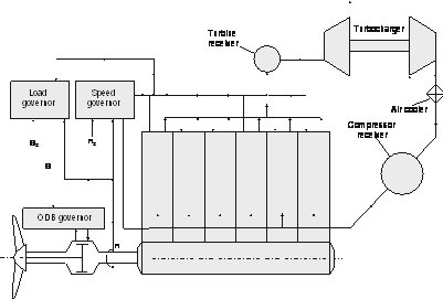
Fig. 1: Propulsion system principal scheme
Mechanical part of the propulsion system in torsional vibration calculation (TVC) is to be modeled as a commonly known N-degree mass-elastic system: the system consisting of lumped masses having specific inertia, connected by the massless stiffness elements.
Motion of the lumped mass k of the system is described by the equation [2]:
\(\displaystyle \frac{d}{{d\phi }}\left[ {\left( {{{J}_{k}}+\Delta {{J}_{k}}(\phi )} \right)\frac{{\omega _{k}^{2}}}{2}} \right]=\sum{{{{M}_{k}}}}\,,\,\,\,\,\,\,\,\,\,\,\,\,\,\,\,\,\,\,\,\,\,(1)\)where \(\displaystyle {{\phi }_{k}}\) – rotation angle; \(\displaystyle {{\omega }_{k}}={{\dot{\phi }}_{k}}\) – angular velocity; \(\displaystyle {{J}_{k}}\) – constant part of the lumped mass inertia;
\(\displaystyle \Delta {{J}_{k}}(\phi )\)– variable part of the lumped mass inertia; \(\displaystyle \sum{{{{M}_{k}}}}\,\)– sum of the torques, applied to the lumped mass.According to [2] equation (1) can be rewritten as:
\(\displaystyle {{\varepsilon }_{k}}\left( {{{J}_{k}}+\Delta {{J}_{k}}(\phi )} \right)=\sum{{{{M}_{k}}}}\,-\frac{{\omega _{k}^{2}}}{2}\cdot \frac{{d\Delta {{J}_{k}}(\phi )}}{{d\phi }}\,\,\,\,\,(2)\)The variable inertia component \(\displaystyle \Delta {{J}_{k}}(\theta )\) inherited mainly to the cylinder lumped mass and the CPP lumped mass. These arise due to the piston and conrod center-of-mass positions changing with respect to the crankshaft axis and due to changing of propeller added inertia during pitch adjusting. See articles [3,4], [5] for appropriate calculation formulas.
Seven categories of the torques contribute to the sum\(\displaystyle \sum{{{{M}_{k}}}}\,\):
- \(\displaystyle M_{k}^{W},\,M_{k}^{J},\,M_{k}^{P}\)- weight, inertia and gas excitation torques are applied to the cylinder lumped masses;
- \(\displaystyle M_{k}^{H},\,M_{k}^{I}\)- hydrodynamic excitation and ice impact torques are applied to the propeller lumped mass;
- \(\displaystyle M_{k}^{D}\)- absolute damping torque is applied mainly to the cylinder and propeller lumped masses;
- \(\displaystyle M_{k}^{E}\)- elastic torque produced by the stiffness elements is applied to all lumped masses.
TVC for open water operation condition when no ice torque is applied usually performed in a frequency domain as steady-state oscillations because shaft rotation speed assumed to be constant as well as the rest propulsion system parameters. Mean torque developed by the engine is in equilibrium with the mean hydrodynamic torque, applied to the propeller.
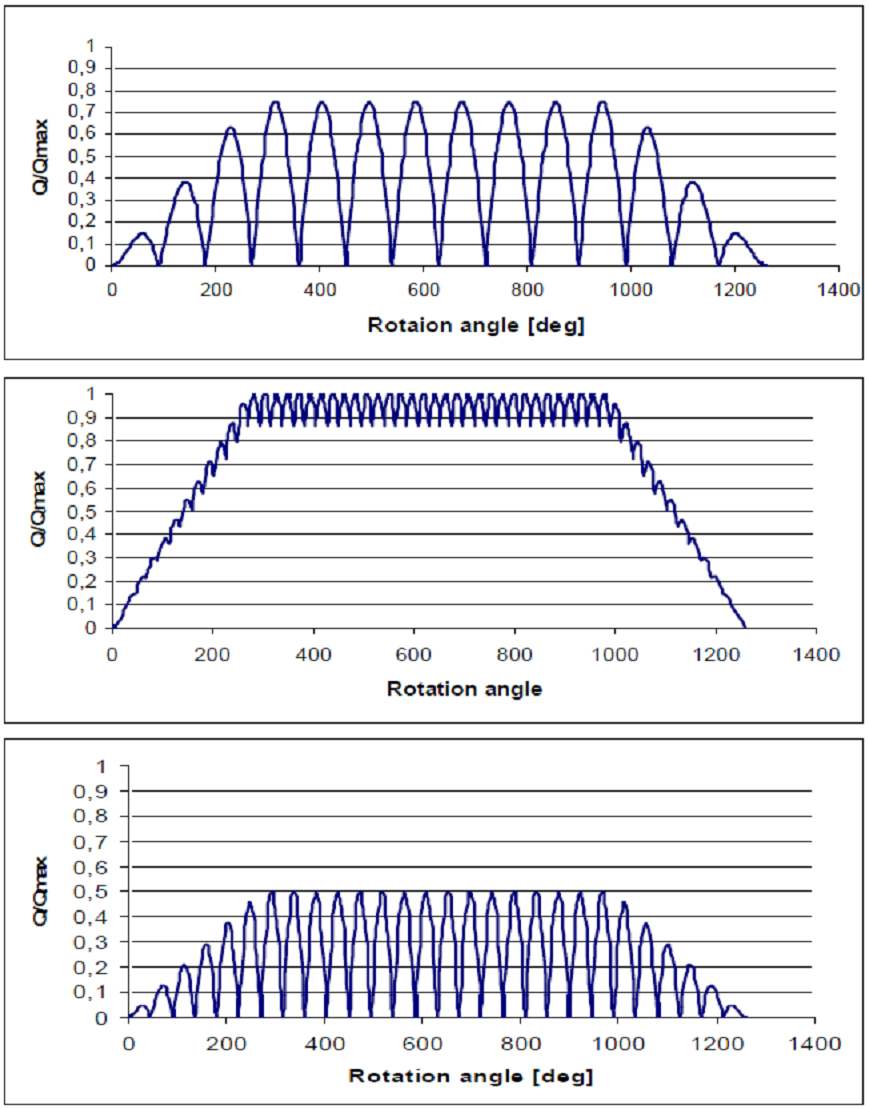
Fig. 2: Ice torque graphs for 4-blades propeller
In ice conditions the torques balance is disturbed by ice impacts. The ice impact torques \(\displaystyle M_{k}^{I}\) in the Classification Rules are described as the sequences of half-sinus waves of blade passing frequency as well as the double frequency. Ice torque graphs for 4-blades propeller at the constant propeller speed are shown in the Fig 2.
Torque amplitude Qmax depends on ship class, propeller and hub diameters and propeller speed.
In the case of ice impacts propeller load changes abruptly that initiate variation of propulsion system parameters. First of all shaft actual speed \(\displaystyle n\) drops and the speed governor increases the components of the fuel supply vector \(\displaystyle \vec{b}\)sequentially to maintain required speed. Where, in spite of maximum fuel supply, the required speed \(\displaystyle {{n}_{z}}\) is not reached, load governor decreases the propeller pitch to decrease ship speed and use the engine energy to overcame ice resistance.
As a result of the fuel supply alteration exhaust gases parameters will alter the combustion air parameters. In total these changes will alter indicating pressure diagram and gas toque component at the cylinder lumped masses [6]:
\(\displaystyle M_{{_{k}}}^{P}=P({{\text{ }\!\!\varphi\!\!\text{ }}_{k}},P_{S}^{*},{{T}_{S}},{{b}_{k}})\cdot F\cdot r\cdot \frac{{\sin ({{\text{ }\!\!\alpha\!\!\text{ }}_{k}}-{{\text{ }\!\!\varphi\!\!\text{ }}_{k}})}}{{\sin {{\text{ }\!\!\alpha\!\!\text{ }}_{k}}}},\,\,\,\,\,\,\,\,\,\,\,\,\,\,\,\,\,\,\,(3)\)where \(\displaystyle P({{\text{ }\!\!\varphi\!\!\text{ }}_{k}},P_{S}^{*},{{T}_{S}},{{b}_{k}})\)– cylinder pressure; \(\displaystyle P_{S}^{*}\)– air receiver pressure; \(\displaystyle {{T}_{S}}\)– air receiver temperature; \(\displaystyle {{b}_{k}}\) – fuel supply vector component in cylinder\(\displaystyle k\);\(\displaystyle F\)– cylinder area; \(\displaystyle r\) – crank radius; \(\displaystyle {{\text{ }\!\!\alpha\!\!\text{ }}_{k}}\)– conrod angle.
For the propulsion shafting transient torsional vibration calculation induced by ice impacts the conventional TVC differential equation system must be expanded with the differential equations for turbocharger rotor (4), turbine receiver (5)-(7) and compressor receiver (8):
\(\displaystyle {{\dot{n}}_{{tc}}}\cdot {{\text{ }\!\!\tau\!\!\text{ }}_{{tc}}}\text{ = }{{f}_{{tc}}}(P_{S}^{*},P_{{tr}}^{*},T_{{tr}}^{*},L_{{tr}}^{{}},m_{{tr}}^{{}},n_{{tc}}^{{}},n),\,\,\,\,\,\,\,\,\,\,\,\,\,\,\,\,\,\,\,\,\,\,\,\,\,\,\,\,\,\,\,\,(4)\) \(\displaystyle {{\dot{m}}_{{tr}}}\cdot {{\text{ }\!\!\tau\!\!\text{ }}_{{tr}}}\text{ = }{{f}_{{mtr}}}(P_{S}^{*},P_{{tr}}^{*},T_{{tr}}^{*},L_{{tr}}^{{}},m_{{tr}}^{{}},n_{{tc}}^{{}},n,\vec{b}),\,\,\,\,\,\,\,\,\,\,\,\,\,\,\,\,\,\,\,\,\,\,\,\,(5)\) \(\displaystyle {{\dot{L}}_{{tr}}}\cdot {{\text{ }\!\!\tau\!\!\text{ }}_{{tr}}}\text{ = }{{f}_{L}}(P_{S}^{*},P_{{tr}}^{*},T_{{tr}}^{*},L_{{tr}}^{{}},m_{{tr}}^{{}},n_{{tc}}^{{}},n,\vec{b}),\,\,\,\,\,\,\,\,\,\,\,\,\,\,\,\,\,\,\,\,\,\,\,\,\,\,(6)\) \(\displaystyle \dot{T}_{{tr}}^{*}\cdot {{\text{ }\!\!\tau\!\!\text{ }}_{{tr}}}\text{ = }{{f}_{T}}(P_{S}^{*},P_{{tr}}^{*},T_{{tr}}^{*},L_{{tr}}^{{}},m_{{tr}}^{{}},n_{{tc}}^{{}},n,\vec{b}),\,\,\,\,\,\,\,\,\,\,\,\,\,\,\,\,\,\,\,\,\,\,\,\,\,\,\,(7)\) \(\displaystyle {{\dot{m}}_{{cr}}}\cdot {{\text{ }\!\!\tau\!\!\text{ }}_{{cr}}}\text{ = }{{f}_{{mcr}}}(P_{S}^{*},m_{{cr}}^{{}},n_{{tc}}^{{}},n),\,\,\,\,\,\,\,\,\,\,\,\,\,\,\,\,\,\,\,\,\,\,\,\,\,\,\,\,\,\,\,\,\,\,\,\,\,\,\,\,\,\,\,\,\,\,\,\,\,(8)\)where \(\displaystyle n_{{tc\,}}^{{}}\)– turbocharger rotor speed, \(\displaystyle m_{{tr}}^{{}}\)– mass of gas in turbine receiver, \(\displaystyle L_{{tr}}^{{}}\)– gas amount in turbine receiver in moles, \(\displaystyle T_{{tr}}^{*}\),\(\displaystyle P_{{tr}}^{*}\)– turbine receiver inhibited flow temperature and pressure,\(\displaystyle m_{{cr}}^{{}}\)– mass of air in compressor receiver; \(\displaystyle \text{ }\!\!\tau\!\!\text{ }_{{tc,\,\,\,}}^{{}}\text{ }\!\!\tau\!\!\text{ }_{{tr}}^{{}}\)– time constants of compressor and turbine receivers; \(\displaystyle f_{{tc,\,\,\,}}^{{}}f_{{mtr,\,}}^{{}}f_{{L,\,\,\,}}^{{}}f_{{T,\,\,\,}}^{{}}f_{{tcr}}^{{}}\)– the right-hand sides functions of the equations [6].
Suitable fuel supply \(\displaystyle {{b}_{k}}\) depends on the normalized torque value \(\displaystyle \text{ }\!\!\mu\!\!\text{ }_{D}^{{}}=\sum{{M_{k}^{P}/{{M}_{{MCR}}}}}\) defined by the speed governor algorithm:
\(\displaystyle \text{ }\!\!\mu\!\!\text{ }_{D}^{{}}=\left\{ \begin{array}{l}1\,\,\,\,\,\,\,\,\,\,\,\,\,\,\,\,\,\,if\,\,\,\,n\,\,\le {{n}_{Z}}-\Delta ,\\\frac{{{{n}_{Z}}-{{n}_{{}}}}}{\Delta }\,\,\,\,\,if\,\,\,\,{{n}_{Z}}>n\,\,>{{n}_{Z}}-\Delta ,\,\,\,\,\,\,\,\,\,\,\,\,\,\,\,\,\,\,\,\,\,\,\,\,\,\,\,\,\\0\,\,\,\,\,\,\,\,\,\,\,\,\,\,\,\,\,if\,\,\,\,n\,\,>{{n}_{Z}},\end{array} \right.\,(9)\)where \(\displaystyle \Delta \)– speed control range, \(\displaystyle {{n}_{Z}}\)– target speed:
\(\displaystyle {{n}_{Z}}=\left\{ \begin{array}{l}{{n}_{Z}}\,\,\,\,\,\,\,\,\,\,\,\,\,\,\,\,\,\,\,\,\,\,\,\,\,\,\,\,\,\,\,\,\,\,\,\,\,\,\text{for}\,\,\mathbf{P}\,\,\text{governor},\\{{n}_{Z}}+\frac{1}{{{{T}_{i}}}}\int\limits_{0}^{t}{{({{n}_{Z}}-n)d\text{ }\!\!\tau\!\!\text{ }\,\,\text{for}\,\,\,\mathbf{PI}\,\,\text{governor},}}\end{array} \right.\)(10) \(\displaystyle {{n}_{Z}}\)– required engine speed.Governor PID algorithm is not effective for low speed installations and does not used here.
2. numerical technique
The choice of the numerical technique for the time-domain solution of the k+5 differential equations described above is a key factor for the successful problem solving. According to the fundamental publication [7] the majority of the numerical algorithms may be collected into the three families – multistage techniques, multistep techniques and optimization techniques.
The disadvantage of the multistage techniques (Runge-Cutta method, Newmark β-method) is that some amount of the additional iterative calculations for every temporal point \(\displaystyle {{t}_{{k+1}}}\) has to be carried out to achieve required accuracy.
The well-known family of the “predictor-corrector” algorithms (Adams-Multon method) belongs to the multistep techniques. The disadvantage of the multistep techniques is that the algorithms could start only from some temporal point \(\displaystyle {{t}_{{s+1}}},\,\,s>1\) but not from the initial point\(\displaystyle {{t}_{0}}\), therefore some other algorithm has to be used at the beginning for the calculations on the initial interval \(\displaystyle [{{t}_{0}};\,{{t}_{s}}]\).
The third family of the optimization techniques is based on the optimization procedures applied to the specified functional \(\displaystyle J(\vec{\theta },\vec{\dot{\theta }},\,\vec{\ddot{\theta }})\), connected to the considered problem. If \(\displaystyle \{{{p}_{n}}\}\) are the set of free unknown parameters in the solution, then the conditions \(\displaystyle {{\partial J}}/{\partial }\;{{p}_{n}}=0\) generate the resulting equations in the algorithm. Different versions of the well-known least-square algorithms are the good representatives of this family [9]. One of them is Kujawski&Gallager method [10], according to which the minimization procedure is formulated as \(\displaystyle {{\partial J}}/{\partial }\;{{\vec{\theta }}_{{k+1}}}=0\) where functional J has to be considered as a square of the total errors of equations for the temporal interval\(\displaystyle [{{t}_{{k-1}}};\,{{t}_{{k+1}}}]\).
To solve the problem of transient torsional vibration problem the Kujawski&Gallager algorithm was specially generalized [11] to be applied to the complete mechanical form of the governing equations with nonlinearities in matrix elements:
\(\displaystyle {\mathrm M}\vec{\ddot{\theta }}+\text{C}\vec{\dot{\theta }}+{\mathrm K}\vec{\theta }=\vec{T}(t)\), (11)where matrices \(\displaystyle {\mathrm M},\,\text{C},\,{\mathrm K}\) are considered as the equivalent inertia, damping and rigidity matrices of the vibration system respectively and \(\displaystyle \vec{T}(t)\) is a vector of generalized excitation forces. For the transient and nonlinear problems some elements of the above mentioned matrices would include dependences of the matrix elements on time, displacement vector \(\displaystyle \vec{\theta }\) and velocity vector\(\displaystyle \vec{\dot{\theta }}\). In this case loading vector may have the same structure too\(\displaystyle \vec{T}(t,\vec{\theta },\vec{\dot{\theta }})\).
The mechanical form of the equation makes the generalised Kujawski&Gallager method most suitable for use together with the finite element method of propulsion shafting modelling [8].
To evaluate the above mentioned techniques four typical algorithms – fourth-order Runge-Cutta algorithm, four-step Adams-Multon algorithm, Newmark β-method and generalized version of Kujawski&Gallager algorithm have been chosen to solve the following differential equations:
1) linear dumping oscillator,
2) nonlinear Duffing’s oscillator and
3) Van-der-Pol’s oscillator with nonlinear damping. Calculations were carried both for free oscillations and for harmonically exited oscillations.
Calculation results brought us to the following conclusion: every of chosen algorithm works correctly for some of the equations and indicates amplitude instability or phase shifting for the rest of the equations. Generalized Kujawski&Gallager optimization algorithm in general showed better characteristics in the comparison to other algorithms.
Hereinafter generalized Kujawski&Gallager algorithm [8,11] is discussed in more details.
At the initial stage of the algorithm, for the constant temporal step \(\displaystyle \Delta t=const\) the second-order polynomial approximation of the solution is applied on the temporal interval \(\displaystyle [{{t}_{{k-1}}};\,{{t}_{{k+1}}}]\) (see Fig. 3):
\(\displaystyle \vec{\theta }\left( t \right)=\left( {L_{t}^{{\left( 2 \right)}}\cdot \vec{\Theta }} \right)=\left( {L_{{k-1}}^{{\left( 2 \right)}}{{{\vec{\Theta }}}_{{k-1}}}+L_{k}^{{\left( 2 \right)}}{{{\vec{\Theta }}}_{k}}+L_{{k+1}}^{{\left( 2 \right)}}{{{\vec{\Theta }}}_{{k+1}}}} \right)\), where \(\displaystyle L_{{k\pm 1}}^{{(2)}}=\pm \frac{1}{2}\tau \left( {1\pm \tau } \right)\) and \(\displaystyle L_{k}^{{(2)}}=(1-{{\tau }^{2}})\) are the Lagrangian polynomials of the second order for local temporal coordinate \(\displaystyle \tau ={{(t-{{t}_{k}})}}/{{\Delta t\in }}\;\left[ {-1,+1} \right]\) and \(\displaystyle {{\vec{\Theta }}_{k}}\equiv \vec{\theta }\left( {{{t}_{k}}} \right)\) are the nodal values of the solution. The same polynomial approximation must be applied for the vector of excitation forces \(\displaystyle \vec{T}(t)=(L_{t}^{{(2)}}\cdot \vec{T})\) in the right-hand side of the equations.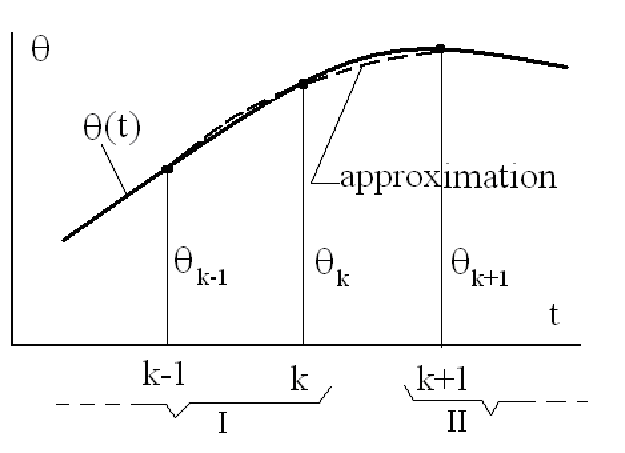
Fig. 3: Approximation of the solution on the temporal interval \(\displaystyle [{{t}_{{k-1}}};\,{{t}_{{k+1}}}]\); I – known portion of the solution, II – unknown portion of the solution.
Approximation generates some errors in the solution or so called “residual forces” in the matrix equations (11)
\(\displaystyle \vec{\Re }\left( t \right)=\left\{ {{\mathrm M}\left( {\ddot{L}_{t}^{{\left( 2 \right)}}\vec{\Theta }} \right)+\text{C}\left( {\dot{L}_{t}^{{\left( 2 \right)}}\vec{\Theta }} \right)+{\mathrm K}\left( {L_{t}^{{\left( 2 \right)}}\vec{\Theta }} \right)-\left( {L_{t}^{{\left( 2 \right)}}\vec{T}} \right)} \right\}\ne 0\)Then, at the second stage of the algorithm [8,11], the functional related to the problem can be formulated as the following:
\(\displaystyle {{J}_{R}}=\int\limits_{{-1}}^{{+1}}{{W\left( \tau \right)\vec{\Re }_{c}^{T}\left( \tau \right){{{\vec{\Re }}}_{c}}\left( \tau \right)d\tau }},\text{ }\) (14)where \(\displaystyle W\left( \tau \right)\) is some weighting function on the considered temporal interval having the properties \(\displaystyle \int_{{-1}}^{1}{{W\left( \tau \right)d\tau =}}1,\,\,\,W\left( {-\tau } \right)=W\left( \tau \right),\,\,\,W\left( \tau \right)>0\) and \(\displaystyle {{\vec{\Re }}_{c}}\left( t \right)=\left\{ {{{{\mathrm M}}_{c}}\left( {\ddot{L}_{t}^{{\left( 2 \right)}}\vec{\Theta }} \right)+{{\text{C}}_{c}}\left( {\dot{L}_{t}^{{\left( 2 \right)}}\tilde{w}\vec{\Theta }} \right)+{{{\mathrm K}}_{c}}\left( {L_{t}^{{\left( 2 \right)}}\tilde{w}\vec{\Theta }} \right)-\left( {L_{t}^{{\left( 2 \right)}}\tilde{w}\vec{T}} \right)} \right\}\)is the vector of residual forces. This vector includes additional weighting factors \(\displaystyle \tilde{w}=diag\left( {{{\alpha }_{{-1}}};\,{{\alpha }_{0}};\,1} \right)\) and estimating of the matrixes \(\displaystyle {\mathrm M},\,\text{C},\,{\mathrm K}\) in some specified point of collocation \(\displaystyle t={{t}_{c}}\in [{{t}_{{k-1}}};\,{{t}_{{k+1}}}]\) (in the case of nonlinear or time-depending elements of matrixes in the equations). Weighting function\(\displaystyle W\left( t \right)\), point of collocation \(\displaystyle {{t}_{c}}\) and weighting factors \(\displaystyle \tilde{w}\) have to be chosen on the next stages of the algorithm.
At the third stage, the algorithm considers \(\displaystyle {{\vec{\Theta }}_{{k-1}}},\,\,{{\vec{\Theta }}_{k}}\) as known values; for the unknown value \(\displaystyle {{\vec{\Theta }}_{{k+1}}}\) we would formulate minimization procedure as the following:
\(\displaystyle \frac{{\partial {{J}_{R}}}}{{\partial {{{\vec{\Theta }}}_{{k+1}}}}}=0\), (15)which finally results in the numerical algorithm:
\(\displaystyle {\vec{\Theta }}_{k+1}=2{{A}^{{-1}}}B{\vec{\Theta }}_{k+1}-\left( {{\mathrm I}-2{{A}^{{-1}}}D} \right) {\vec{\Theta }}_{k+1}+\Delta {{t}^{2}}\left[ {{{A}^{{-1}}}E\left( {{{{\vec{T}}}_{{k+1}}}+{{{\vec{T}}}_{{k-1}}}} \right)-2{{A}^{{-1}}}\left( {G{{{\vec{T}}}_{k}}+H{{{\vec{T}}}_{{k-1}}}} \right)} \right]\) (16)
where \(\displaystyle k=1,2,3,….\) and for the first temporal point \(\displaystyle {{t}_{1}}\) it modifies to the equation:
\(\displaystyle {{\vec{\Theta }}_{1}}={{\left( {A-D} \right)}^{{-1}}}\left[ {B{{{\vec{\theta }}}_{0}}+\Delta t\left( {A-2D} \right){{{\vec{\dot{\theta }}}}_{0}}+\left( {\frac{1}{2}E{{{\vec{T}}}_{1}}-G{{{\vec{T}}}_{0}}} \right)} \right]\)(17)where \(\displaystyle {{\vec{\theta }}_{0}},\,{{\vec{\dot{\theta }}}_{0}}\) are the initial values of the problem solution.
The following expressions for the matrices A, B, D, E, G, H are used:
\(\displaystyle \left. \begin{array}{l}A=\left\{ {{\mathrm M}_{c}^{T}} \right.{{{\mathrm M}}_{c}}+\Delta t{\mathrm M}_{c}^{T}{{\text{C}}_{c}}+\Delta {{t}^{2}}{{k}_{1}}\left( {{\mathrm M}_{c}^{T}{{{\mathrm K}}_{c}}+{\mathrm K}_{c}^{T}{{{\mathrm M}}_{c}}+2\text{C}_{c}^{T}{{\text{C}}_{c}}} \right)+\\\,\,\,\,\,\,\,\,\,\,\,\,\,\,\,\,+\frac{1}{2}\Delta {{t}^{3}}{{k}_{1}}\left( {{\mathrm K}_{c}^{T}{{\text{C}}_{c}}+2\text{C}_{c}^{T}{{{\mathrm K}}_{c}}} \right)\quad \left. {+\Delta {{t}^{4}}{{k}_{2}}{\mathrm K}_{c}^{T}{{{\mathrm K}}_{c}}} \right\}\ ,\\B=\left\{ {{\mathrm M}_{c}^{T}} \right.{{{\mathrm M}}_{c}}+\Delta {{t}^{2}}\left( {{{k}_{3}}{\mathrm M}_{c}^{T}{{{\mathrm K}}_{c}}+{{k}_{1}}{\mathrm K}_{c}^{T}{{{\mathrm M}}_{c}}+2{{k}_{1}}\text{C}_{c}^{T}{{\text{C}}_{c}}} \right)+\\\text{ +}\left. {\Delta {{t}^{4}}{{k}_{4}}{\mathrm K}_{c}^{T}{{{\mathrm K}}_{c}}} \right\}\,\,,\\D=\left\{ {\Delta t{\mathrm M}_{c}^{T}{{\text{C}}_{c}}+\frac{1}{2}\Delta {{t}^{3}}{{k}_{1}}\left( {{\mathrm K}_{c}^{T}{{\text{C}}_{c}}+2\Lambda _{c}^{T}{{\text{C}}_{c}}} \right)} \right\}\ ,\\E=\left\{ {{{k}_{1}}{\mathrm M}_{c}^{T}+\Delta t{{k}_{1}}\text{C}_{c}^{T}+\Delta {{t}^{2}}{{k}_{2}}{\mathrm K}_{c}^{T}} \right\}\ ,\,\,\,G=\left\{ {{{k}_{3}}{\mathrm M}_{c}^{T}+\Delta {{t}^{2}}{{k}_{4}}{\mathrm K}_{c}^{T}} \right\}\ ,\,\\\,H=\left\{ {\Delta t{{k}_{1}}\text{C}_{c}^{T}} \right\}.\end{array} \right\}\ \)(18)The algorithm includes four unknown weighting factors \(\displaystyle {{k}_{j}},\,\,j=1,2,3,\,4\) which are some integrals from weighting function \(\displaystyle W\left( \tau \right)\) and approximation polynomial\(\displaystyle L_{k}^{{(2)}},\,L_{{k+1}}^{{(2)}}\). These factors must be estimated by the application of the algorithm to some model problem, associated with the main problem.
Linear damping oscillator \(\displaystyle \ddot{u}+2\nu \dot{u}+\omega _{0}^{2}u=0\ ,\,\,\,\,t>0\) with the initial conditions \(\displaystyle u(0)=1,\,\,\,\dot{u}(0)=0\) can be used as a model problem for transient torsional vibration calculation.
Applying the algorithm to the model problem we would take into account the accuracy conditions for the first temporal point \(\displaystyle {{t}_{1}}\) and stability conditions at the infinity\(\displaystyle {{t}_{n}}\to \infty \). Application of these conditions generates finally the following results for the weighting factors \(\displaystyle {{k}_{j}},\,\,j=1,2,3,\,4\) [11]: relations between the factors
\(\displaystyle \left. \begin{array}{l}{{k}_{1}}=\frac{1}{2}\kappa ,\text{ }{{k}_{3}}=\frac{1}{2}\left( {\kappa -\left( {1+{{\chi }_{0}}} \right)} \right)\,\,;\,\\{{k}_{2}}=\kappa \left( {1+{{\chi }_{1}}} \right)+{{k}_{4}}-\frac{1}{{24}}\left( {1+{{\chi }_{2}}} \right),\end{array} \right\}\) (19)accuracy and stability conditions for two free tuning factors \(\displaystyle \kappa ,\,\,{{k}_{4}}\) \(\displaystyle \left. \begin{array}{l}\frac{5}{{12}}\kappa \left( {1+{{\chi }_{3}}} \right)+{{k}_{4}}\left( {1+{{\chi }_{0}}} \right)-\frac{7}{{180}}\left( {1+{{\chi }_{4}}} \right)=0,\\1+2\left( {\kappa -\frac{1}{6}} \right)\Delta \omega _{*}^{2}+\left[ {{{k}_{4}}+\kappa \left( {\kappa -\frac{1}{{12}}} \right)} \right]\Delta \omega _{*}^{4}+\\\text{ }+\left[ {{{k}_{4}}+\frac{1}{4}\left( {\kappa -\frac{1}{{12}}} \right)} \right]\left( {\kappa -\frac{1}{{12}}} \right)\Delta \omega _{*}^{6}\ge 0,\end{array} \right\}\) (20)
where \(\displaystyle {{\chi }_{j}},\,j=0,\ldots ,4\) are some correction factors related to the damping effects in the model problem and \(\displaystyle \Delta \omega _{*}^{2}=\Delta {{t}^{2}}(\omega _{0}^{2}-{{v}^{2}})\).

Fig. 4: Stability diagram for tuning factors \(\displaystyle \kappa ,\,\,{{k}_{4}}\): \(\displaystyle 1,\ldots ,5\) – the upper boundaries of conditional stability for values \(\displaystyle \Delta {{\omega }_{*}}=1.0;\,\,1.25;\,\,1.60;\,\,1\,.80;\,\,5.0\) respectively; 6 – eighth-order accuracy condition for testing problem: \(\displaystyle {{k}_{4}}+\frac{5}{{12}}\kappa +\frac{7}{{180}}=0\); /////// – domain of the absolute stability; the specific points on the diagram: A – \(\displaystyle \left(\kappa = \frac{1}{{24}} ,\,\, {{k}_{4}} = \frac{1}{{48}}\right)\); B – \(\displaystyle \left(\kappa = 0 ,\,\, {{k}_{4}} = \frac{1}{{4}}\right)\); C – \(\displaystyle \left(\kappa = \frac{1}{{4}} ,\,\, {{k}_{4}} = -\frac{1}{{24}}\right)\).
The accuracy and stability conditions in equation (20) can be displayed on the algorithm stability diagram for the testing problem, Fig. 4. This diagram may be used to specify two free weighting factors \(\displaystyle \kappa ,\,\,{{k}_{4}}\) in the solution of the actual problem. For example in the first approach the values \(\displaystyle \kappa = \frac{1}{{24}} ,\,\, {{k}_{4}} = \frac{1}{{48}}\) can be adopted in the calculations.
3. CALCULATION SAMPLE
Calculation algorithm is intended to be implemented in ShaftDesigner software [12] as a separate module for transient ice impact torsional vibration analysis. Currently this module does not take into account shaft speed drop due to the ice impacts. Some calculation results for IACS polar class PC1 vessel, equipped with low speed installation are discussed below.
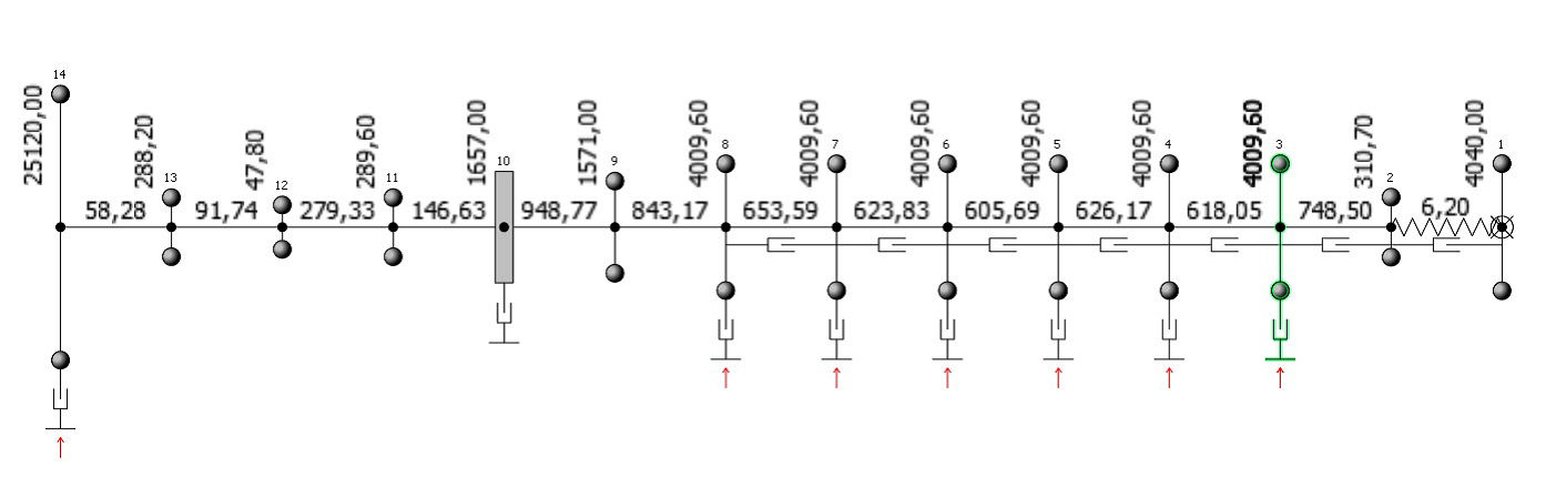
Fig. 5: Mass-elastic system for low speed installation
Main characteristics of the propulsion installation are as the following:
Engine stroke 2
Cylinder number 6
MCR 5000 kWt
Rated speed 109 rpm
Propeller type FPP
Blade number 4
Propeller shaft diameters 410/130
Steady vibration stress in the propeller shaft and in the throw 6 (aftermost cylinder marked as lumped mass 8) for open water operation condition are shown in the Fig. 6 and Fig 7.

Fig. 6: Steady vibration stress in the propeller shaft
For both elements the maximal torsional vibration stress 8.5-16.8 MPa arise within speed interval 60-75 rpm. Vibration stress component of order 6 prevail in the synthesis stress.
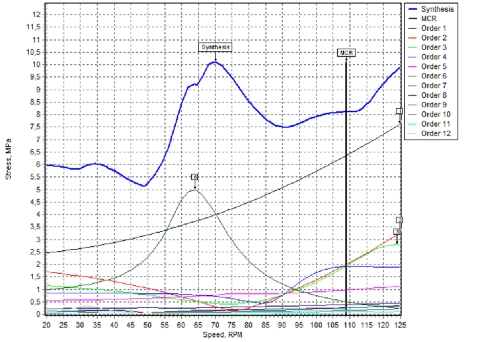
Fig. 7: Steady vibration stress in the throw 6
The transient vibration stress during ice milling is much higher: 165-348 MPa for the propeller shaft (Fig. 8) and 51-96 MPa for the throw 6 (Fig. 9).
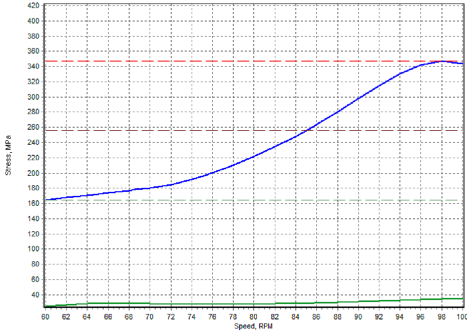
Fig. 8: Transient vibration stress in the propeller shaft
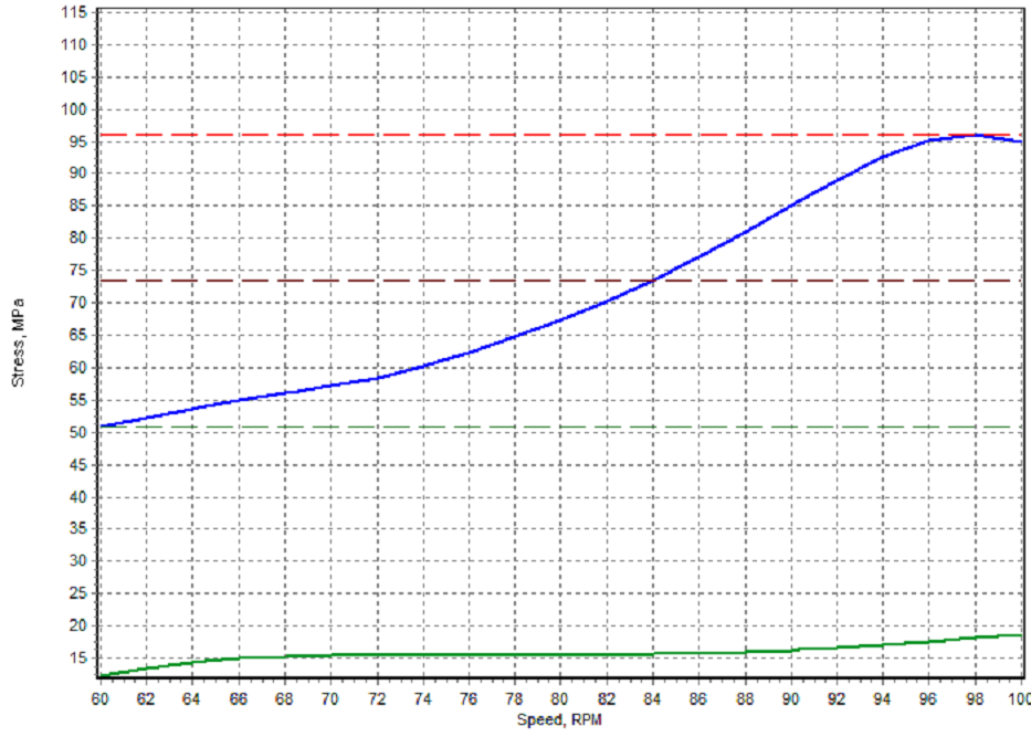
Fig. 9: Transient vibration stress in the throw 6
Maximum torsional stress due to the ice impacts, in contradistinction to open water condition, arise within the speed interval 95-100 rpm. It is exactly the same interval where the first-blade order resonance is located (see order 4 curve in the Fig. 6). Classification societies recommend analyse torsional vibration due to the ice impacts at this location first of all.
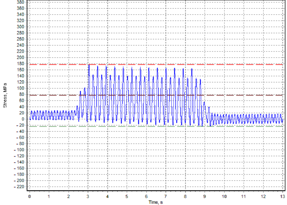
Fig. 10: Transient vibration propeller shaft stress at 68 rpm
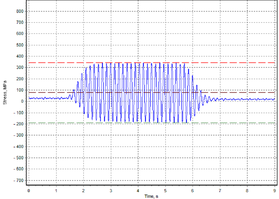
Fig. 11: Transient vibration propeller shaft stress at 100 rpm
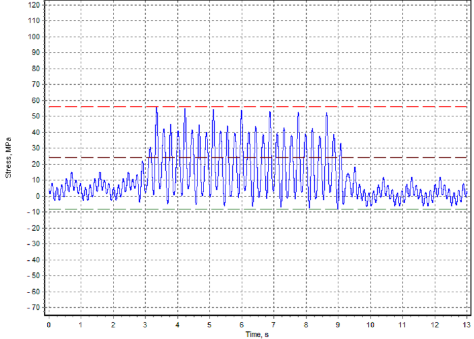
Fig. 12: Transient vibration stress in the throw 6 at 68 rpm
In the Fig. 10-13 transient torsional vibration graphs are shown. As can be seen ice impact torsional stress decay very fast after ice torque becomes equal to zero.
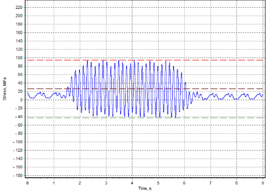
Fig. 13: Transient vibration stress in the throw 6 at 100 rpm
CONCLUSIONS
Proposed algorithm was programmed and included to ShaftDesigner CAE package as a separate module for transient torsional vibration calculation. Applications of this module demonstrate quite acceptable calculation time for full mass-elastic system. Hence no simplification of mass-elastic system is required to calculate transient torsional vibration in ice operating conditions.
As a first stage of algorithm implementation shaft speed drop was not taken into account. Such option gives the possibility for the fast evaluation of torsional vibration stress because it does not require of whole propulsion shafting system modelling. It is a decisive argument at the early stage of propulsion shafting design. In addition using this option we are on the safe side. It means that if the calculated parameters satisfy the acceptance criteria, more detailed calculation may not be required at all.
The option for the whole propulsion system modelling is under testing now. It will be useful when the fast modelling results do not satisfy acceptance criteria or real propulsion system parameters are of interest. In the last case the realistic not statutory ice torques are desirable to have as an input.
ACKNOWLEGMENTS
We express special thanks to Stanislav Avanesov and Erik Werner of Germanischer Lloyd for their contributions and feedback.
REFERENCES
1. Ice strengthening of propulsion machinery, 2010 DNV Classification Notes No 51.1, September, 63 pp.
2. Frolov К.V., Popov S.А., Мusatov А.К., and others., 1987, Mechanisms and Machines Theory – Мoscow: «Vysshaya Shkola», 496 pp. (in Russian)
3. Hesterman D.C., Stone B.J., 1994, A Systems Approach to the Torsonal Vibration of Multi-Cylinder Reciprocating Engines and Pumps. Proceedings of the IMechE, Part C: Journal of Mechanical Engineering Science 208 (6), pp. 395-408.
4. Guzzomi A.L., 2007, Torsional Vibration of Powertrains: An investigation of Some Common Assumptions. PhD thesis, University of Aestern Australia. 136 pp.
5. MacPherson D.M., Puleo V.R., Packard M.B., 2007, Estimation of entrained water added mass properties for vibration analysis. SNAME New England Section, June.
6. Тarasenko А.I., 2008, Non-linear Dynamic Model of Low Speed Marine Engine. Vestnik Dvigatelestroyeniya: Zaporzhzhia: ”Мotor Sich”, 3 (20), pp. 202–205. (in Russian)
7. Hull G., Watt J.M., 1976, Modern Numerical Methods for Ordinary Differential Equations, Clarendon Press. Oxford, 312 pp.
8. Brebbia C.A., Walker S., 1979, Dynamic Analysis of Offshore Structures. London-Boston, 230 pp.
9. Eason E.D., 1984, A review of list-squares methods for solving partial differential equations. Trans. Soc. Math. Eng. 1, pp. 1021-1046.
10. Kujawski J., Gallager R., 1985, An efficient higher order algorithm for nonlinear transient dynamic analysis. Proceed. NUMETA – 85 Conference Swansea, pp. 51-58.
11. Serdjuchenko A.N. Dynamics of waves and ships in sea conditions including nonlinear effects. Applied Hydromechanics, Vol. 72. Kiev, pp. 112-135 (in Russian)
12. Y. A. Batrak., 2009, New CAE Package for Propulsion Train Calculations, ICCAS papers, September Shanghai, v II, pp.187-192.